Course outline:
part I
- introduction to RAD-seq assembly
- ipyrad installation and command line (CLI)
- In depth look at the parameters
- introductory tutorials with CLI
part II
- introduction to Python, jupyter, and reproducible analyses
- introduction to parallel computing in Python
- ipyrad Python code (API) and the ipyrad environment
- empirical data examples
- empirical downstream analysis examples
1. Introduction to RAD-seq assembly
- Short reads (usually 50-150bp) single or paired.
- Loci usually align perfectly, not tiled into contigs.
- SNP data including full sequence data.
- usually ~1e3 - 1e6 loci.
- phased SNPs within loci, not phased between loci
- anonymous (denovo) or spatial-located (reference-mapped)
Available assembly software
- Standard reference-mapping approaches (BWA + Picard + GATK + ...)
- STACKS
- pyRAD)
- TASSEL-UNEAK
- ipyrad
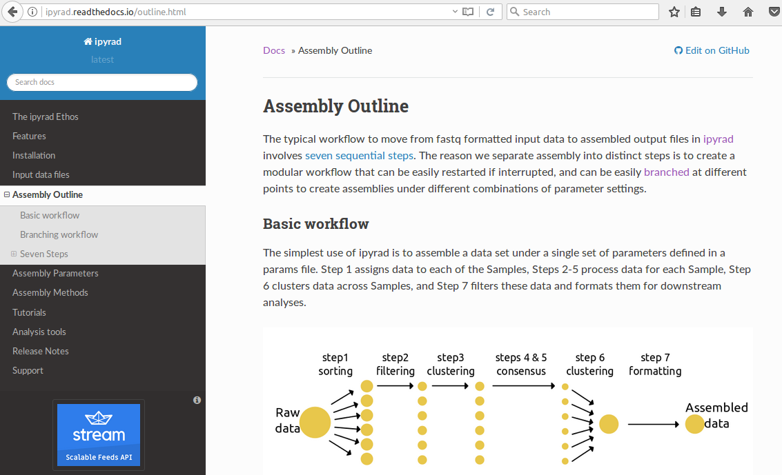
The general workflow:
- Separate reads among sampled individuals based on a barcode or index.
- Trim and filter reads based on quality and adapter contamination.
- Identify alleles or read copies based on sequence similarity (clustering or mapping).
- Make consensus base and haplotype calls based on clustered reads.
- Identify orthology by clustering haplotypes across samples.
- filter for paralogs, junk, etc. and write output files.
Advantages to using ipyrad over the other methods:
- Provides denovo, reference, and denovo+reference hybrid assembly methods.
- Includes alignment steps to allow for indel variation.
- Fast and massively parallelizable (hundreds/thousands of cores)
- Low memory footprint, e.g., compared to stacks.
- Branching methods support reproducibility and exploring parameter settings
- Python API supports integration with Jupyter and scripting.
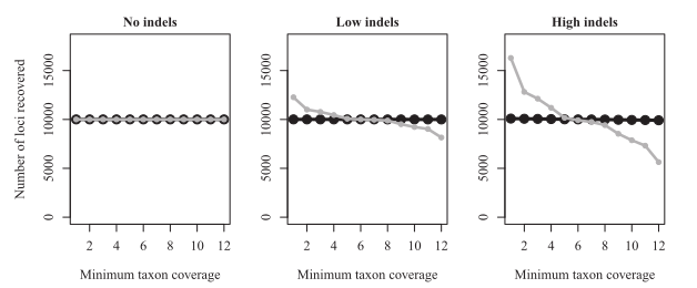
Important differences of large effect:
- Indels are present (loci are split b/c variation looks like frame-shift)
- reads are different lengths (from trimming or different sequencing runs)
- ipyrad treats paired-reads as a linked haplotype (Stacks treats them as two separate loci)
- ipyrad can trim & filter your data appropriately for the datatype.
- ipyrad can cluster with reverse-complement matching (e.g., pairGBS data)
- parallelization over multiple hosts/nodes is easy.
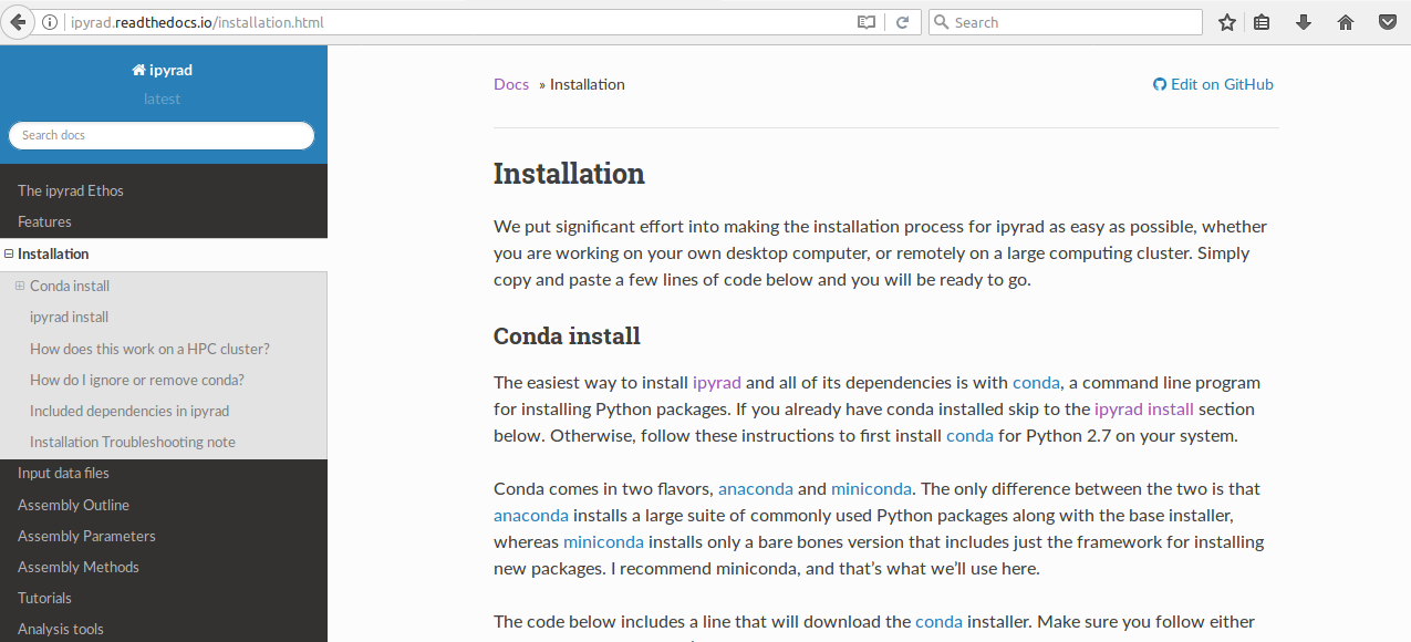
Installation
We will use the conda software installation tool to install all of our software locally.
Common mistakes when installing conda
- make sure you choose the correct version (OSX vs Linux)
- make sure you answer yes when it asks if you want to install it
- make sure you call '
source ~/.bashrc' after installation
## example argument entry to conda
# conda install -c <channel> <package-name>

## install software from my channels
conda install -c ipyrad ipyrad
conda install -c eaton-lab toytree

## install raxml from the commonly used channel bioconda
conda install -c bioconda entrez-direct sratools
We'll return to conda later to install more software.
The ipyrad command-line (CLI)
And introduction to the ipyrad setup and parameter settings.
Entering parameters
Create an empty params file with default values by calling ipyrad with the -n command.
Entering parameters
Use a text-editor, such as nano, to enter new values into the params file.
Running ipyrad (command line)
- You must always specify a params file with
-p. - To run steps of the assembly use
-s. - To see a stats summary use
-r - Use
-hto see several other commands.
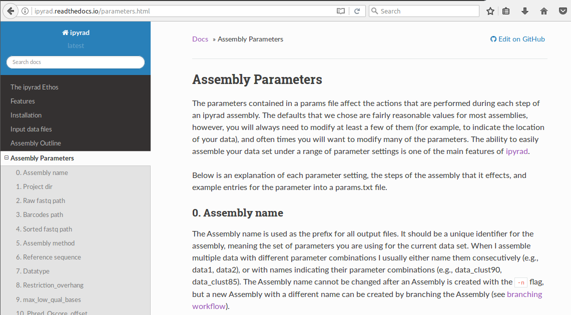
3. The parameters of ipyrad


4. Introductory tutorials

1. Python, jupyter, and reproducible science
- Widely used in big-data science (Google, Facebook, Github, etc.)
- Many libraries link compiled code-base (e.g., Numpy, Scipy, Theano)
- Easy integration with databases (e.g., HDF5, MYSQL)
- Just-in-time compilation (Numba library)
- Easy code-sharing/reproducibility/exploring with Jupyter
But is it fast enough?
- Scripting language (The glue that ties together higher level code)
See a great Pycon keynote address on this topic here (I mean, watch it later if you're interested.)
What should reproducible science look like?
- Easy to reproduce the software environment & versioning (e.g., conda)
- Not using a GUI (unfortunately)
- Easy to access the original data (e.g., directly from online archives)
- Easy to read and understand code (markdown documentation and clean code)
- Parameters of methods/software are displayed (not hidden)
- Easily accessible (e.g., Github, Zenodo)
- Executable
An example we will reproduce today:
http://nbviewer.jupyter.org/github/dereneaton/ipyrad/blob/master/tests/cookbook-empirical-API-1-pedicularis.ipynb
Published examples from my own work:
https://github.com/dereneaton/RADmissing
https://github.com/dereneaton/virentes
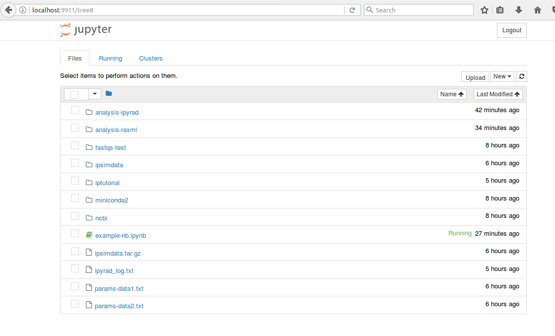
Running jupyter-notebook locally
When you call jupyter from a terminal it will start a notebook server, which you can access through your browser to send and receive data with computing kernels to run code and display its output (e.g., Python, R, Julia, or bash).
## call this command from a terminal on your laptop
jupyter-notebook
Running jupyter-notebooks remotely
This can be a little tricky, but once you figure it out it is very rewarding. You can leave the notebook running on a cluster, and connect to when you want to run analyses, disconnect, and reconnect later. This link provides a more in-depth description with a short video tutorial (with sound) for doing this same thing through a job submission script on a cluster. But for now, just run the commands below on the MBL cluster.
This should be run on the cluster (remote)
## first, let's make a password for our notebook
jupyter-notebook password

## Next, launch a notebook server with this command
jupyter-notebook --no-browser --ip=$(hostname -i) --port=$(shuf -i8000-9999 -n1)
Look at the output of the notebook server, it will list a port number that was randomly selected (this is to avoid ya'll using the same port) and it will show an ip address (e.g., 127.0.1.1).
This should be run on your laptop (local)
## on your laptop (local) call this command
## ssh -N -L port:ip:port user@login
ssh -N -L 8888:127.0.1.1:8888 deaton@class05.jbpc-np.mbl.edu
2. introduction to parallel computing in Python
ipyrad makes use of the ipyparallel library for large-scale parallel computing which is particularly designed for interactive parallel computing in jupyter notebooks.
## start a cluster with all available cores
ipcluster start

## start a cluster with N cores
ipcluster start --n=4

## start a cluster with a specific name and settings
ipcluster start --n=4 --profile='deren'

## start a cluster that will connect to all cores on multiple hosts
ipcluster start --n=80 --engines=MPI --ip=*
When ipyrad connects to the ipcluster instance you can see details of the connection.
import ipyrad as ip
import ipyparallel as ipp

## connect to client
ipyclient = ipp.Client()

## print client info
ip.cluster_info(ipyclient)
The general approach is to distribute work among the kernels (engines), wait for them to finish, and then collect the results. All of this happens under the hood in ipyrad, but a simple understanding of it helps to understand how to easily parallelize any type of code within a jupyter-notebook.
def f(x):
    return x + 10

## send a job to the cluster
async = ipyclient[0].apply(f, 10)

## wait for job to finish before leaving loop
while 1:
    if async.ready():
        break

## print result
print 'result is', async.result()
3. The ipyrad API
## an Assembly object
data = ip.Assembly("example")

## the parameters
data.set_params("project_dir", "tutorial")
data.set_params("sorted_fastq_data",
                "/class/molevol-shared/ipyrad-tutorial/fastqs-Ped/*.gz")

## run the analysis on a specific cluster
data.run('1', ipyclient=ipyclient)
## branch and subsample
subsamples = [i for i in data.samples if "prz" not in i]
sub = data.branch("sub", subsamples=subsamples)

## branch and change params over a range of values
assemblies = {}
for ct in [0.80, 0.85, 0.90, 0.95]:
    newname = "clust_{}".format(ct)
    newdata = data.branch(newname)
    newdata.set_params("clust_threshold", ct)
    assemblies[newname] = newdata
## split an Assembly into two groups
allsamples = data.samples.keys()
data1 = data.branch("data1", allsamples[:5])
data2 = data.branch("data2", allsamples[5:])

## set different params on each assembly
data1.set_params("mindepth_statistical", 10)
data2.set_params("mindepth_statistical", 5)

## run each Assembly
data1.run("5")
data2.run("5")

## merge the samples back into a single Assembly
full = ip.merge("full", [data1, data2])
full.run("67")
4. Empirical data examples
Open the link below for one of the following notebook. They're very similar, the first is a group of plants, the second is a group of birds, so choose your favorite. We will then each create a new notebook from scratch by copy/pasting code from these notebooks to produce our own new analysis notebook (run either on your laptop or on the cluster).
5. Empirical downstream analyses
The ipyrad analysis toolkit provides additional downstream formatting and filtering of data sets, as well as wrapper tools that allow running external software in efficient and reproducible ways.
## the general design of analysis tools
import ipyrad.analysis as ipa

## initate an analysis object with a name, data file, and other args
r = ipa.raxml(
    name="example",
    data="analysis-ipyrad/output.phy",
    *args)

## see and change the object.params
r.params

## run command to execute the code or send to client
r.run(ipyclient)
useful examples
- iterating over K values in structure and replicates within Ks
- iterating over priors in BPP, and replicates, or doing thermodynamic integration
- or, simply saving yourself time in typing the same arguments many times (e.g., raxml)
Success
You are now ready to go on and assemble RAD-seq data sets to your very specific and particular needs, and to keep a very detailed record of what you did to share with your friends and cruel reviewers.
Final advice:
- Look at your data!
- Explore your assembly (different parameters)
- Run exploratory analyses (structure, raxml)
- Keep yourself organized.